GUI User Guide¶

The graphical user interface to the BASIL tools can be accessed by typing asl_gui at the command line. It should provide most of the options required for analysis of ASL data inlcuding the majority of the more advanced features of BASIL.

Note: if you are using a release of BASIL that you have installed separately from FSL you may need to specfically call asl_gui with the full path to: where it is installed: e.g. /Users/{blah}/Downloads/oxford_asl/asl_gui. This page documents the GUI avilable in FSL v6 (also available via the pre-release website), there are some differences with the GUI found in FSL v5.

The GUI largely provides a more approachable interface to the oxford_asl command line tool (and even produces a command line call for oxford_asl for you to reuse separately if you like).

The GUI has five tabs, whose function are fairly self-explanatory. Each tab represents one step in the (notional) workflow for your ASL analysis and you can work through them using the prev/next buttons in the lowe right of each tab. For many analyses you will be able to accept many of the default options and you might find you do no need to even visit some of the later tabs.

Input Data: Specify details of the ASL data here, this is also where oyu have to record details about the acquisition used.
Calibration: Specify your calibration image (if you have one), to be used to produce images of absolute perfision (in ml/100g/min). You can also choose to set options relating to the method for estimation of the equilibrium magnetization of arterial blood.
Structural: Specify a structural image, or the output of a previous run of fsl_anat, to be used in the analysis process and for registration. Analysis can proceed without a structural iamge, but if you have one it is recommeded that you include it.
Distortion correction: If you have suitable images to do distortion correction of your ASL data you can include them here.
Analysis: Options relating to the analysis, primarily the kinetic model and the estimation process.

More details on each tab are provided below. Note that some of the options available on each tab depend on what information is present in your data (set on the data tab). Thus your view of the tab might differ from the one shown here slightly.

Input Data¶

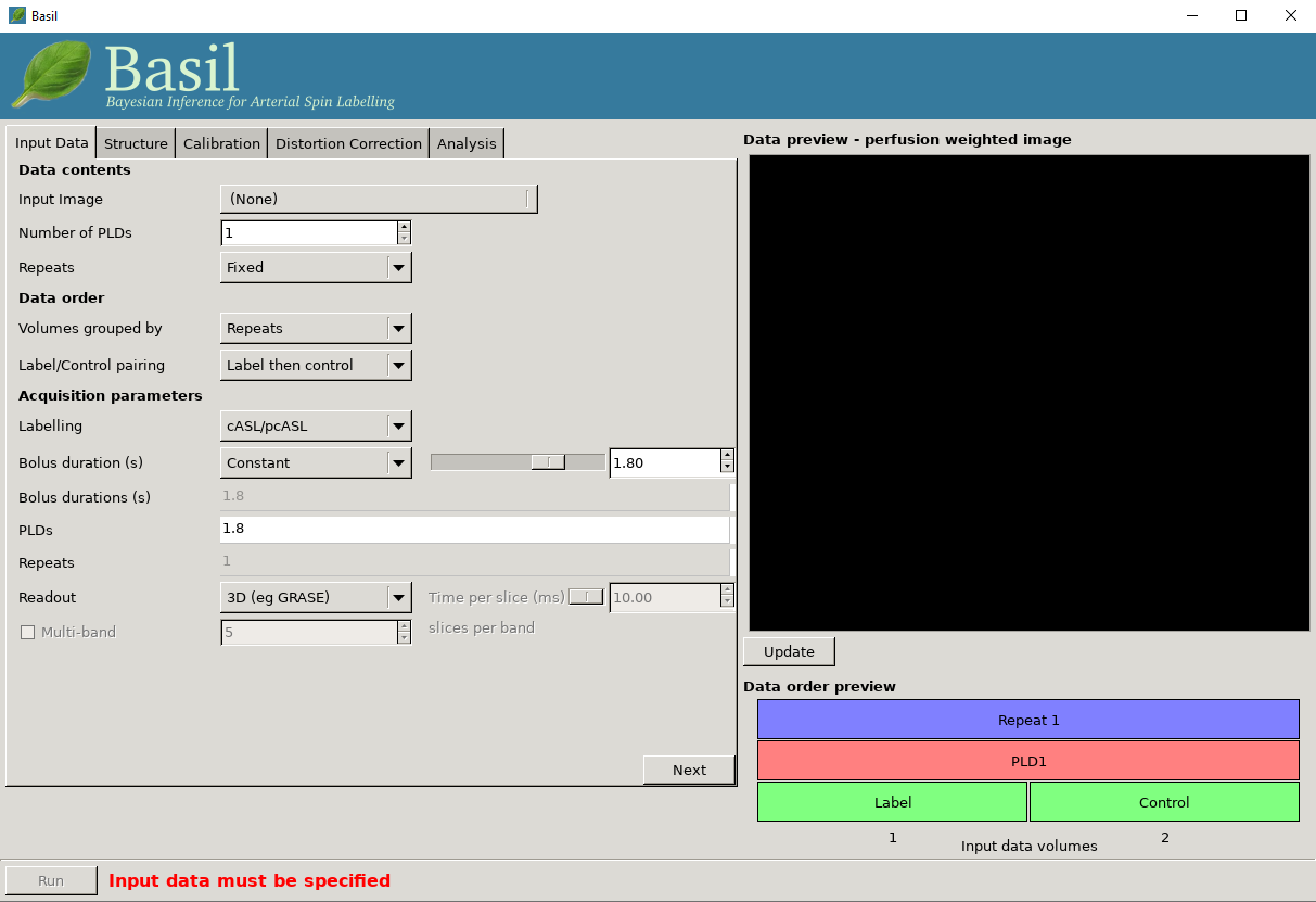
Data contents

Input Image: A single 4D nifti file of the main ASL data (either label-control pairs or subtracted images), with the individual measurements in the 4th dimension.
Numer of PLDs: Set the number of post-label delays (or inversion times/inflow times) in the data.
Number of repeats: A value will be calculated here based on the number of PLDs you entered in the box above. Use this is a sanity check again the number of repeats you expect from your acquisition.

Data order

Volumes grouped by: For multi-PLD data, this specifies whether the acquisition consisted of a full set of all PLDs, with the whole block repeated multiple times (Volumes grouped by Repeats), or if the first PLD was repeated multiple times, followed by all repeats of the second PLD, and so on (Volumes grouped by TIs/PLDs).
Label/control pairing: This specifies whether the label image was before the control or vice versa, or if the data is already subtracted.

The choices selected here are reflected in the data order preview view, at the bottom right of the window. This gives a visual representation of the volumes in the input data. The horizontal axis represents the sequence of volumes in your data, and the boxes above shows the PLD, repeat and label/control corresponding to each volume.

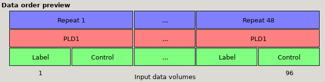
Data preview for single-PLD data with Label then control ordering and 48 repeats. Note that the ‘Volumes grouped by’ option makes no practical difference for single PLD data.

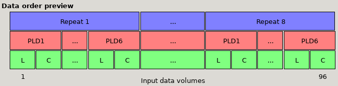
Data preview for multi-PLD data with 6 PLDs, with Label then control ordering and volumes grouped by Repeats. The first set of volumes contains a single repeat of all the PLDs, followed by another block of all PLDs, etc.

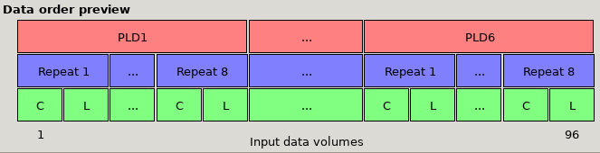
*Data preview for multi-PLD data with 6 PLDs, with Control then label ordering and volumes grouped by PLDs. Note that the order of the label and control images (the green L and C boxes) has changed, and the first set of volumes is 8 repeats of PLD1, followed by 8 repeats of PLD 2, etc.

Acquisition parameters

Labeling: Choose the labelling scheme employed, either pcASL/cASL or pASL (note for analysis purposes there is no difference between cASL and pcASL).
PLD / TIs: Set the post-labeling delay(s) (or inversion time(s)) for the acquisition. For a multi-PLD/TI acquisition there will be a value to be set for each PLD/TI in the data.
Bolus duration (s): The duration of the labeled bolus in seconds.

[Advanced] If your data is multi-PLD you can additionally specify different bolus durations for the different PLD, by changing from single to mulitple. Using this option you can have any combination of PLD and bolus duration to match those used in the acquisition
Readout: Specify if a full 3D or a 2D multi-slice acquisition was used. For 2D you should then set the time taken to acquire each slice (in miliseconds) as this determines the true PLD/TI for each slice.
Multi-band: Inlcude this option where the readout was a multi-band (simultaneous multi-slice) 2D acquisition, in which case you need to specify the number of slices in each band, to correctly set the PLD/TI for each slice.

Data preview - perfusion weighted image

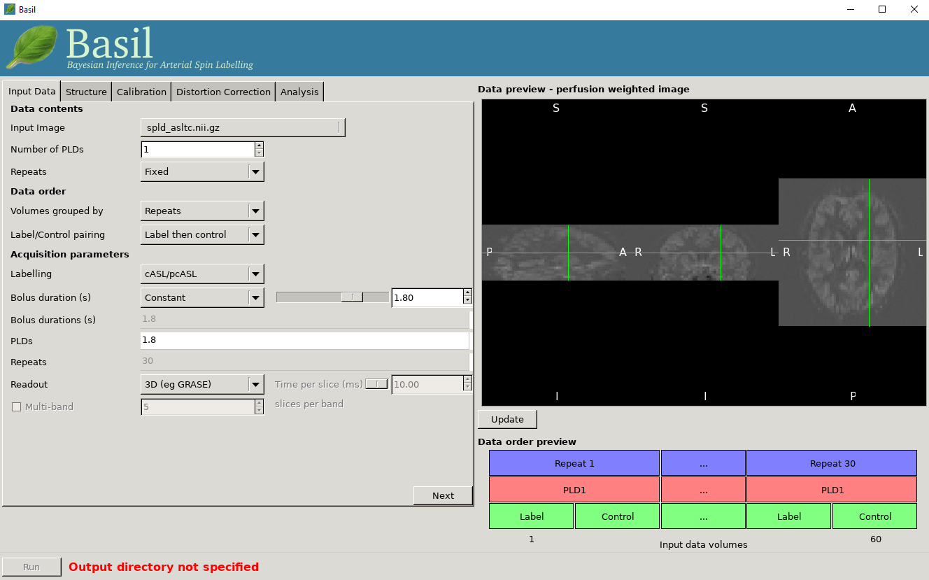
On the right of the window is a preview pane. Once you have set the Data contents and Data order parameters you can press preview and the GUI will generate a perfuion-weighted image based on the information you have provided. This is a good sanity check to ensure that you have set these parameters correctly - if at this stage you dont see something that looks like a perfusion-weighted image - i.e., something in which the grey matter structure of the brain is evident - then you probably haven’t set the ordering correctly. You can scroll through the slices in the image using your mouses’ scroll wheel (or equivalent). Note that for multi-PLD data this preview averages all the different PLD.

Structural¶

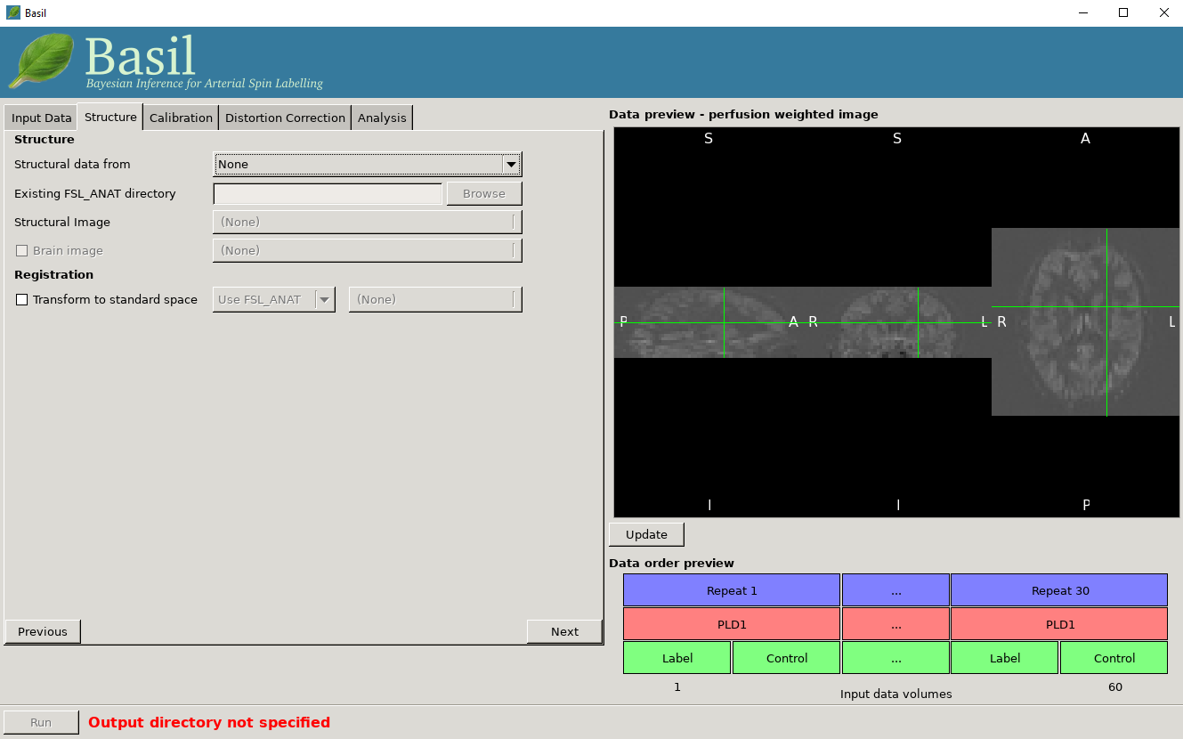
Structural Data From - The recommended option is Existing FSL_ANAT output where you have already run FSL_ANAT on the structural image. Select the FSL_ANAT output directory below. Alternatively you can supply a structural image and run FSL_ANAT on it as part of the analysis, however this will add quite a lot of runtime so it’s better to do it once and then just re-use the output. You can also avoid using FSL_ANAT at all and just supply your own structural image. If you have a brain segmentation you can supply it (otherwise BET will be run), and you can supply an existing transformation to standard (MNI) space (either a linear FLIRT matrix transformation or a nonlinear FNIRT warp).

Calibration¶

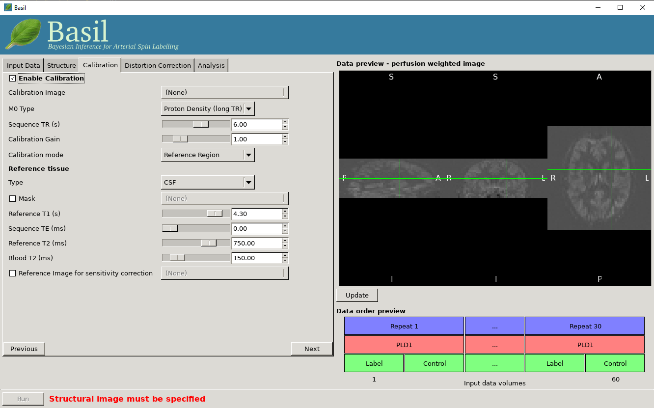
Enable Calibration

Note you specfically have to chose the option to enable calibration. It is possible to perform ASL analysis without calibration, but only then posisble to get relative perfusion images.

Calibration image: An image to be used for calibration. This should have the same resolution as the ASL data, ideally have the same readout, and be proton density weighted.
M0 type: Specify what sort of calibration image you are supplying. In most cases this will be Proton Density, unless you have data with a pre-saturation in which case chose saturation recovery.
Sequence TR (s): The repetition time of the sequence used to colelct the calibration image (this may not be the same as the ASL data itself). This is used to correct for non-equilibrium effects on the PD image.
Calibration gain: If there is a difference in acquisition gain between the calibration image and the ASL data it can be set here. This might be the case where background suppression has been applied for the main ASL data.
Calibration mode: Chose either to compute and apply the calibration factor (equilibirum magnetization of arterial blood) voxelwise, or from within a Reference Region. The latter relies upon a structural image being provided (unless you supply your own mask for this below), the former is the approach assumed by the white paper.

Reference tissue

These options apply to the Reference Region mode of calibration.

Type: The reference tissue type to use, one of: CSF/white matter/grey matter/none. For the first three options a mask will be generated automatically from the structural image (if you have specfied one), otherwise (or alternatively) you should specify your own mask in the Reference Tissue Mask box (this should be in the same space as the ASL data). Generally CSF or white matter are good choices, avoid grey matter due to partial volume effects.
Sequence TE: This corrects for T2 differences between the reference tissue and the brain tissue (using a blood T2 value) based on the TE of the data (which is assumed to be the same as any calibration image).
Reference T1: T1 of the reference tissue.
Reference T2/Blood T2: T2 values, these are only relevant if you specify the TE of your sequence. T2 of the reference deafults to a CSF value. These should be replaced by T2* values if appropriate.

Distortion Correction¶

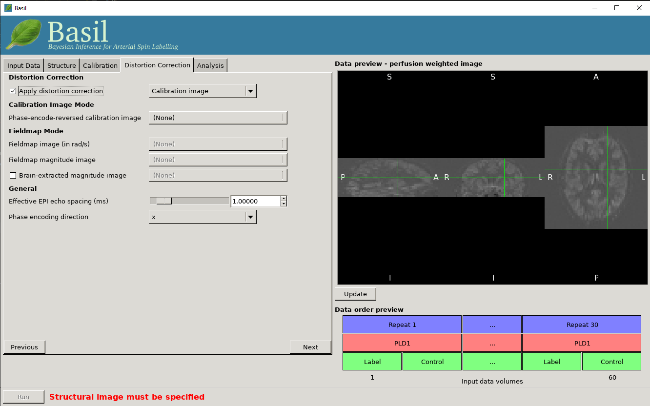
Apply distortion correction: Select to apply correction for readout distortions in the ASL data using a suitable set of reference images. You will need either a calibration image with a different phase encoding direction to the main calibration image, or a fieldmap.

Calibration image mode

Phase encode reversed calibration image: An image that matches the calibration image in all acquisition parameters, except that the phase-encode direction is reversed.
Effective EPI echo spacing: Set this value from the sequence in seconds (typical values are of the order of 0.01 ms).
Phase encode direction: The phase encode direction of the calibration image (i.e. the image entered on the Calibration tab) and must match that of the main ASL data.

Note that in this mode oxford_asl uses TOPUP to do the distortion correction. For this, the Effective EPI echo spacing is converted to total readout time by multiplication by the number of slices (minus one) in the encode direction.

Fieldmap mode

Effective EPI echo spacing: Set this value from the ASL sequence in seconds (sometimes called the dwell time), typical values are of the order of 0.01 ms.
Phase encode direction: The phase encode direction of the ASL images (entered on the Calibration tab).
Fieldmap image: A fieldmap image (need not necessarily matched to the ASL nor structural image resolution) in rad/s - be careful about the units, as this is not consistent between neuroimaging tools.
Fieldmap magnitude image: A magntiude image to go with the fieldmap, this is used for registration of the fieldmap.
Brain extracted fieldmap magntiude image: Brain extracted version of above image.

For more information on fieldmapping see the documentation associated with FUGUE (note the fieldmap correction in the BASIL GUI is akin to using FEAT for fieldmap correction and uses epi_reg, albeit in a way specfically setup for ASL data). A common choioce for phase encoding is Anterior Posterior (AP), which would normally tranlsate into ‘y’. However, whether this is ‘+y’ or ‘-y’ isn’t necessiarly preditable and you might need to try both and see which one visibly makes the distortion worse (and then use the other!)

Analysis¶

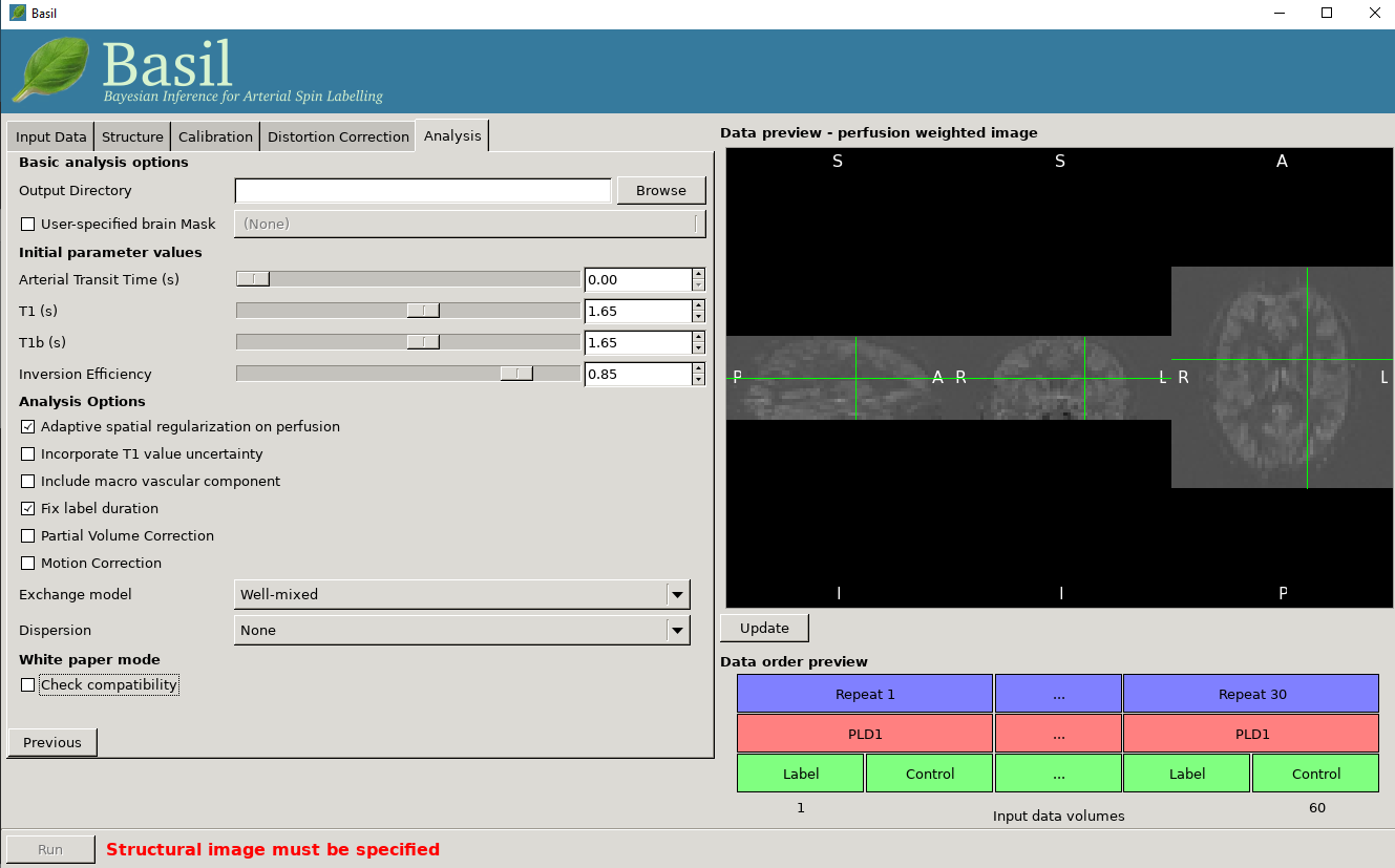
Basic analysis options

Output directory: where to put the results.
User-specified brain mask: Normally, BASIL will try to create a brain mask for you using the available data, however you may specify your own mask here (in the same space as the ASL data).

Inital parameter values

This section sets parameter values for the kientic model. In some cases these are treated as initial and/or prior (mean) values, but are also estimated in the analysis itself.

Arterial Transit Time: The assumed value for the ATT. For multi-PLD ASL, ATT is estimated from the data and this value is used as prior information, for single delay data this value will be treated as fixed. The default 0.7 appears to be reasonable for pASL, but longer values ~1.3s have been found to be more suitable for pcASL data, these are the defaults used by the GUI. (in white paper mode this value is set to 0)
T1/T1b: T1 values for tissue and blood. Defaults are 1.65 seconds for blood and 1.3 seconds for tissue (based on 3T field strength). (In white paper mode both T1 values are set to 1.65 seconds).
Inversion efficiency: A fixed value for the inversion efficiency applied in the calculation of absolute perfusion. The default values (0.85 for pcASL and 0.98 for pASL) are taken from the white paper.

Analysis Options

Adaptive spatial regularisation on perfusion: applys a spatial prior to the perfusion image during estimation, thus making use of neighbourhood information. This is a highly recommended option, and is on by default.
Incorporate T1 uncertainty: Permits voxelwise variability in the T1 values, this will primiarly be reflected in the variance images for the estimated parameters, dont expect accurate T1 maps from conventional ASL data.
Include macro vascular componet: Corrects for arterial or macrovascular contamination, and it suitable where the data multi-PLD (even where flow suppresion has been applied).
Fix label duration: Takes the value for the label duration from the Input Data tab as fixed, turn off to estimate this from the data (the value on the data tab will be used as prior information in that case). You are most likely to want to deslect the option for pASL data, particularly where QUIPSSII/Q2TIPS has not been used to fix the label duration.
Partial Voume Correction: Correct for the different contributions from grey and white matter, and CSF to the perfusion image. This will produce separate grey and white matter perfusion maps.
Motion Correction: Uses mcflirt to perform motion correction of the ASL data (and the calibration image).
Exchange/Dispersion model: These are advanced options that affect the modelling of the blood/tissue compartments and the dispersion of the labelled blood bolus during transit.

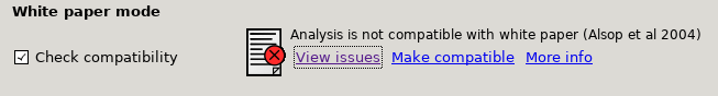
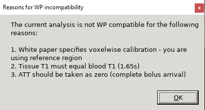
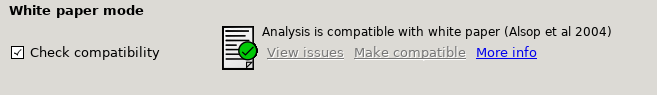
White paper mode

This option allows you to check if the analysis you have set up is compatible with the recommendations in the consensus paper (Alsop et al, 2014). This paper described a simple kinetic model for ASL analysis primarily designed for single-PLD data. While BASIL is capable of more complex modelling, particularly for multi-PLD data, it may be useful for comparison to be able to perform an analysis that uses the white paper recommendations. Selecting this option allows the user to view and correct their options for this purpose.

Output¶

The outputs from the GUI are a perfusion image called perfusion.nii.gz, which provides blood flow in relative (scanner) units, and an arrival time image called arrival.nii.gz for multi-PLD ASL. If a calibration image has been provided then a further image, perfusion_calib.nii.gz, is also produced, which is a flow map in absolute units (ml/100g/min). Results in native ASL, structural and standard space will appear in the output directory within separate subdirectories. Where applicable transformation between spaces will also be saved, along with summary measures of perfusion in the native_space subdirectory if the structural information is availabe to calculate these.

If calibration was performed then a separate subdirectory will be created and will contain text file called M0b.txt that records the estimated M0 value from arterial blood if the reference region mode was use, otherwise an image will be supplied instead. For reference region calibration, if a manual reference tissue mask was not supplied then the automatically generated one will also be saved in as refmask.nii.gz, you should inspect this to ensure that it is a reasonable mapping of the tissue you are using for the reference region (normally CSF in the ventricles).